SSA transformation for GHC's native code generator (Part 2)
SSA based Live Range Discovery
In the first part, I explained the motivation to bring SSA-transformation to GHC’s NCG. Here, I want to look at the implementation challenges, decisions and results.
SSA in the Backend
I’ve used pseudo-code in the first part, but generally, you’ll have some intermediate representation (IR) in your compiler, which is in SSA.
For example, a three address code (TAC), where each instruction represents an operation,
taking two input arguments and one output argument, e.g., IADD x, y, z -> z = x + y.
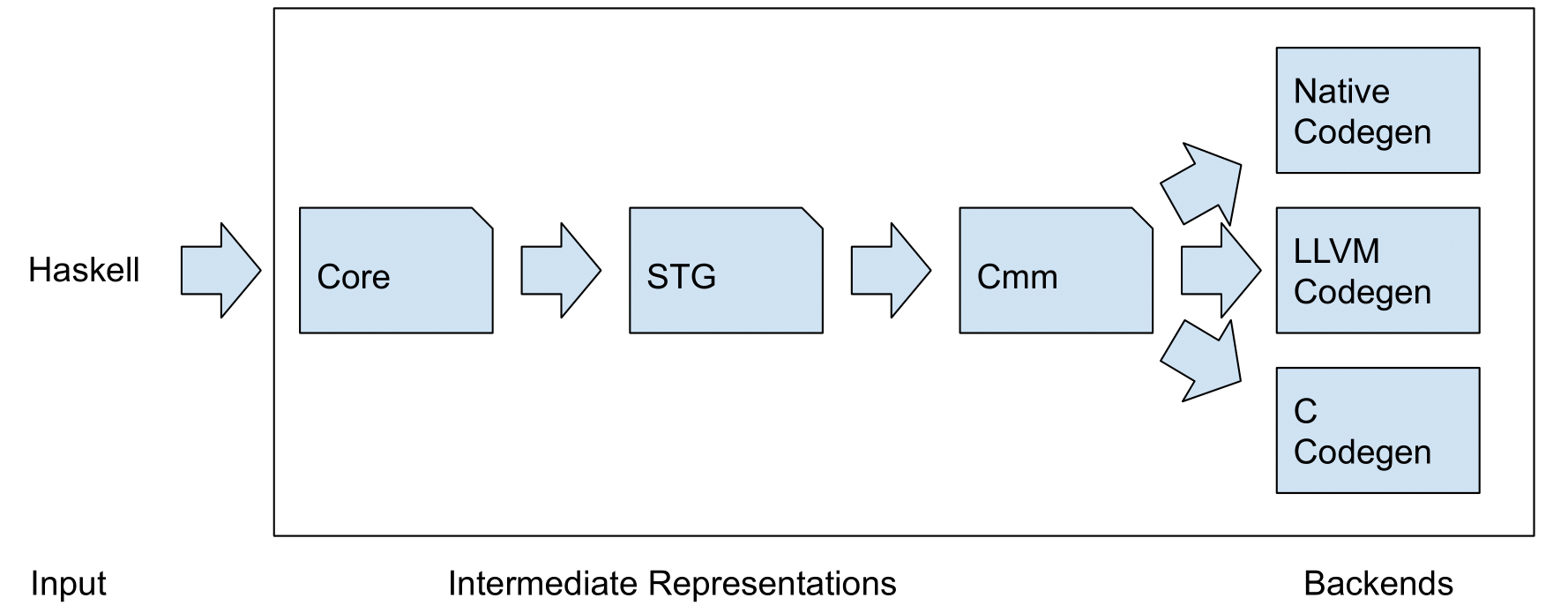
Modern compilers usually use multiple IRs, adapted to different compilation phases and tasks. They may or may not be in SSA. GHC has been around for a while and has several compilation phases and IRs. I won’t describe them here in detail1, but they are Core, STG, C–. C– is a low-level, imperative language with an explicit stack. NCG performs instruction selection on C– and spits out machine instructions for the selected platform. So at this point, we’re not dealing with an IR anymore2.
There are actually quite a few challenges when trying to implement SSA-form on machine instructions.
Pre-colored Registers
Sometimes, the ISA or ABI requires you to use certain registers in specific places.
For example, the x86_64 calling convention requires the passing of function arguments in
specific registers.
Or think about special purpose registers, like the x86_64 stack registers RBP and RSP.
Instruction selection already emits these physical register references where necessary. Obviously, we can’t promote these to SSA variables and start renaming them willy-nilly. In this case, i.e., for live range discovery, we can simply get a way with ignoring them all together, since we are not moving any code3. (FYI, this will be a common theme in the following subsections.)
Modifying and 2-Address Instructions
Most real world ISAs have the annoying property of not being neat, regular and simple.
x86 has many instructions that modify an operand (i.e., in and out operands).
Let’s say %v1 denotes a virtual register number 1, then inc %v1 increments %v1,
or v1 := v1 + 1.
Another example is the two-address addition instruction: add %v1, %v2 is %v2 = %v1 + %v2.
This is clearly not in SSA, as we are producing a value but we can’t assign a new name! One may introduce an intermediate representation to handle this case, constraining the in-out operand pair together somehow - but again, in our use case, we can ignore this!
If we only care about live ranges having unique vreg names, this is OK because the in-out operand pair belongs together anyway. There is no way we could assign different registers here.
Conditional Instructions
Some architectures have conditional (or predicated) instructions, which will only execute,
if a specific condition is met, i.e., normally some status bits must be set in a status register.
For example, x86_64 offers the cmov, or conditional move instruction.
As an example, CMOVE %v1, %v2 is equal to if (x == y) { v2 := v1 }.
32-Bit ARM can basically make every instruction predicated, whereas AARCH64 dialed that down a bit.
I’m not going to discuss their benefits or drawbacks, but since NCG supports architectures with these instructions, we need to take them into account. Again, I’m choosing the most simple route. I consider them non-kill definitions and don’t rename their target.
Further Reading
If you’d like to read more about these challenges, then check-out the SSA Book and “Using the SSA-Form in a Code Generator” by Benoît Dupont de Dinechin.
Implementation
Let’s get down to business. The ticket tracking the implementation can be found here.
Overview
The general workflow, including the new SSA transformation, is as follows and can be found in CmmToAsm.hs:
Instruction Selection -> Liveness Analysis -> SSA Construction -> SSA Destruction -> Register Allocation
For construction, I employed the classic Cytron et al. algorithm4 and destruction handled in the simplified fashion outlined in the first part. I’m constructing pruned-SSA, i.e., only insert φ-nodes for values that are actually live and used. This yields fewer φ-nodes and only “productive” ones, that I can use to find all the webs. But to get that information, I’ve plugged the SSA-steps after the existing Liveness Analysis. That is a classic data-flow analysis, i.e., a fixed-point algorithm.
Modelling Data
Since I didn’t want to rewrite large parts of the code generator, I had to stay close to the original data types in a way.
I’m greatly simplifying here, but basically, after liveness analysis, a procedure is list of strongly connected components (SCCs) of basic blocks:
[SCC (LiveBasicBlock instr)]
We have our LiveIn-Sets, i.e., sets of vregs live on the entry of a basic block, in the main procedure structure (and we need those to place only live φ-functions).
The LiveBasicBlocks contain the ID (or label) of the block and a list of instructions with liveness information (which vregs are read/written/modified, are born/die).
SCCs are either acyclic, i.e., just one block, or they are CyclicSCCs, containing a list of blocks.
The cyclic SCCs are the top-level loops in a procedure (and may contain more loops).
I’m not really interested in the SCC structure, as I need the Control Flow Graph (CFG) anyway, as it is more complete and lets me access all the connections directly, without having to navigate lists and find jumps “manually”. N.B., the CFG in the backend is currently only supported for x86_64, that’s why I can’t support SPARC or PowerPC. I’m not sure what the status for the new AARCH64 support is.
For the construction algorithm, I need random access, so I’m putting everything into a map. But I need to be able to rebuild the exact same SCC-based structure after destruction, otherwise I can’t reuse the rest of the backend. To achieve that, I’m wrapping each block with information telling me, which SCC it belongs to and I’m using a “deterministic map”, which preserves iteration order:
type BlockLookupTable instr
    = UniqDFM BlockId (SccBits (SSABasicBlock instr))

data SccBits a
    = AcyclicBit a | CyclicBit Int a

data PhiFun = PhiF RegId RegId [RegId]
          -- ^ oldId newId args

data SSABasicBlock instr
    = SSABB [PhiFun] !(LiveBasicBlock instr)
For example:
[A -> B -> [C -> D -> E] -> F -> [G -> H]]
turns into:
[A: A, B: B, C: 1 C, D: 1 D, E: 1 E, F: F, G: 2 G, H: 2 H]
Construction
I don’t want to go into great detail here, as better descriptions of the Cytron et al. algorithm can be found in many compiler textbooks (e.g., “Engineering a Compiler”) or online. There may also be better algorithms around (see “Conclusion”).
The gist is, you need to compute the dominance frontiers to know where to place φ-functions and then you need to start renaming definitions in a depth first pre-order walk over the CFG.
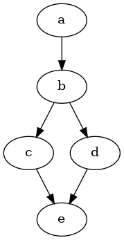
One node d in a directed graph is said to dominate a node n, if every path from the start node to n must go through d. Every node d dominates itself, but d is said to strictly dominate n if d dominates n and d ≠ n. The dominance frontier is the set of nodes, that d just doesn’t dominate, i.e., if d dominates an immediate predecessor of n, but does not strictly dominate n itself, it is in the dominance frontier.
Looking at the graph below, we can see that b dominates both c, d and e - to reach them, you must go through b. But c and d do not dominate e (only themselves). e is in the dominance frontier of c and of d and a block, where we may have to place a φ-node. Looking at the graph, we can intuitively see that, as two conflicting variable definitions from c and d would reach e and we’d need to reconcile them.
Whether we actually need a φ-function here, depends on whether there really was a live variable at that point in the original program. If we bother to check that, we get pruned-SSA. Otherwise it would still be called minimal-SSA, as that only requires that we place φs at join points and not everywhere (which would lead to very pointless and inefficient maximal SSA).
For the renaming part, you need to manage some state and stacks of current names for the current “level” of the CFG you are on. This has actually proven to be the most expensive part of the whole algorithm.
If you are interested in details, check out the relevant chapters in “Engineering a Compiler”, the code or my bachelor’s thesis.
Evaluation
To evaluate my changes, I let them loose on GHC’s nofib benchmark suite, looking both at spill statistics and perf numbers. I compared both the linear scan and the graph coloring allocators with and without SSA transformation.
Graph coloring register allocators use a heuristic to decide, which live range to spill once no more free registers are available.
-fregs-graph uses a very simple one - it just spills the longest live range.
This works surprisingly well (I tested it against some other ones, before my SSA implementation), but my hunch is, that this has something to do with vregs representing disjoint live ranges, making them longer on average.
Therefore, I also implemented a simple Chaitin-style spill heuristic.
Looking at more sophisticated spill heuristics in combination with SSA-transformation may be worthwhile.
Unique vregs
The point was to verify my theory, that most programs contain disjoint live ranges with the same vreg name.
The median increase in unique vreg names, across all benchmarks, is 5.44%, with the single largest increase being 21.04%.
I looked at the results for the real group in detail and all programs showed an increase, except for the tiny programs in real/eff.
Spills - The Good
Spills are both loads and stores. But register-register moves (reg-reg moves) are also noteworthy. Even though they are a metric used in papers, their cost seems to have gone down quite a bit over the last decades. Most modern desktop CPUs contain a much larger register file internally, than just the architectural registers (16 for x86_64). So they can apply register renaming in their execution pipeline. It’s like switching the label in a shelf, instead of moving the merchandise lying there.
I’ve also added SPILLS*, where I am excluding never spilling programs. Since I’m looking at just the relative changes in spills, programs that spilled zero times across all runs only distort the picture.
| graph-ssa | |||
|---|---|---|---|
| Spills | Spills* | reg-reg moves | |
| Median | 0% | -20.00% | -5.40% |
| graph-chaitin-ssa | |||
| Median | Spills | Spills* | reg-reg moves |
| 0% | -24.54% | -5.67% |
The changes for the linear scan allocator are less impressive:
| linear-ssa | |||
|---|---|---|---|
| spills | spills* | reg-reg moves | |
| Median | 0% | -1.09% | 0% |
Runtime - The Bad
OK, so reducing spills is great and all, but what really matters are actually executed instructions. After all, you could remove all spills from rarely executed straight line code and it wouldn’t add up to anything, compared to a hot loop containing spill code.
The results here are not overwhelming.
I’ve added all three columns to the same table, but the graph-* columns are measured against -fregs-graph baseline, whereas ‘linear-ssa’ is measured against the linear scan allocator baseline.
The numbers are relative changes in CPU cycles as reported by perf.
| graph-ssa | graph-chaitin-ssa | linear-ssa | |
|---|---|---|---|
| Geo. mean | -0.47% | -0.74% | 0.20% |
| Median | -0.31% | -0.39% | 0.08% |
| Weighted Avg. | -0.96% | -1.10% | 0% |
So what does this mean? Nofib-compare gives you the geometric mean. I wanted to explore some other averages, because there is, unfortunately, a huge difference in runtime of the benchmark programs. That is not intentional, they are supposed to have similar lengths, but they drift over time. I included the weighted average (weighted by fraction of total runtime), because there are many programs that run for a few milliseconds on one end of the spectrum and one benchmark takes 58 seconds to complete on my machine. You just can’t compare that. The short program is so much more sensitive to interferences and 5% change of 200ms vs 58000ms can’t be lumped together, IMHO.
Alright, so what does that leave us with?
If the results are correct, we might expect around 1% improvement for -fregs-graph and basically nothing for linear scan.
Depending on the cost, I’d take 1%, since for compiler engineers working on mature compilers, 1-2% is already a win.
I tried to drill down a bit in my thesis to explain some of the results, but I’m not a 100% sure.
A hand full of results weren’t really stable across runs. Some seem to be due to higher cache misses (spill code placement and even changes in code layout can have that effect).
Generally, I think that there are still so many things that can be improved in -fregs-graph, but live range renumbering seems to be a prerequisite anyway.
So what about linear scan? I’m less familiar with that algorithm and code, but I have a hunch. Linear scan will make allocation decisions going through the code and insert “fix-up” code/blocks when assigned registers have to be changed. If I understand that correctly, you are not constrained to assign only one real register to a given vreg and most of the fix-up code will be reg-reg moves (but spills are needed too). That would mean, that renumbering just isn’t such an issue to begin with and since reg-reg moves are mostly quite cheap, even the cases where it would lead to more code are not so bad.
If you are interested in the raw numbers, they can be found in the ticket and a more lengthy discussion of the results can be found in my thesis.
Compile times - The Ugly
OK, I said I would take a speedup of 1%, but only at an adequate cost.
You see, I knew this wouldn’t be fast. We are doing strictly more work.
The only gains would be fewer iterations of register allocation (for -fregs-graph only) and possibly a speedup by a faster compiler compiled with that new optimization.
I’ve also used pretty basic algorithms and I only tuned them ever so slightly.
(Plus I’m not an experience Haskell developer and I have no intuition on how to write well performing Haskell.)
Alright, so, the slowdown I have observed compiling Cabal was almost… 30%. That is absolutely terrible, I’m not going to lie. I got some feedback on my code and tried a few things, but it barely made a dent.
But fret not, not all is lost.
Conclusion
-fregs-graph could need some love, there is no renumbering step and SSA transformation not only could take care of that, but it could also enable future optimizations.
My implementation (hopefully) shows, that there is some room for this, but that the improvement is not guaranteed to be large and cost must be low.
-fregs-graph itself could see better results with a different spill heuristic (possibly) and some other improvements (coloring for spill slots? memory addressing instead of stores/loads?).
There are a few possible optimizations for my SSA transformation pass. But several people have let me know, that a better, more modern algorithm exists5. I’m looking into implementing that algorithm and placing it before liveness analysis. Then I can do that on SSA-form directly, where I don’t need to run analyses in a loop until a fixed-point is reach, due to the SSA properties (so that’s supposed to be faster). But the current liveness analysis also removes some dead code as well - so I just need to take a look at the current code and the papers and make sure that I produce correct code.
What excites me quite a bit more though, is the possibility of writing a new graph-based register allocator that operates on SSA directly. Work on bringing register allocation to SSA form has been done and the discovery of some interesting properties made in the last two decades.6 So my next big project will be a new graph coloring register allocator on SSA-form for GHC!
If you spot any mistakes, omissions or want to provide feedback, comments, questions - you can reach me on Twitter, or via mail with my username at gmail.
-
I recommend Takenobu’s GHC Reading Guide for an overview. ↩
-
Well, there are still a few meta-instructions, like SPILL and LOAD, but all-in-all it’s pretty close to assembly. ↩
-
I think one could promote them to a distinct class of SSA variables and store a mapping to the original register. ↩
-
The description in “Engineering a Compiler” is great, as per usual. ↩
-
Braun et al. - “Simple and Efficient Construction of Static Single Assignment Form” ↩
-
See Hack06 for graph coloring on SSA and Wimmer&Franz2010 for linear scan on SSA ↩