SSA transformation for GHC's native code generator (Part 1)
Improving the Graph Coloring Register Allocator
For my first big project on GHC, I wanted to try and improve the Graph Coloring Register allocator in NCG (GHC’s Native Code Generator), aka -fregs-graph.
When code generators emit instructions, they usually use an unlimited number of virtual registers (vregs) and map those to physical registers (or real regs), possibly after changing the code around with optimizations. This register allocation step is generally one of the last ones and extremely important for performance. Registers are a scarce resource and memory access is orders of magnitude slower.
Two of the dominant paradigms for register allocation are Graph Coloring1 based and Linear Scan2 register allocators.
These have been around since the eighties, respectively nineties, but are still highly relevant and in wide use.
Generally speaking, graph coloring based approaches are supposed to yield better quality code, but take more time and memory,
whereas linear scan is faster, at a cost of quality.
GHC currently only uses a (very good) linear scan based allocator, since -fregs-graph has been suffering from bad performance since ca. 2013.
So looking at AndreasK’s improvement ideas, I chose to try live range splitting.
Live Ranges and Graph Coloring
I’m borrowing the definition of live range from Cooper & Torczon’s “Engineering a Compiler”, chapter 13:
A single live range consists of a set of definitions and uses that are related to each other because their values flow together. That is, a live range contains a set of definitions and a set of uses.
Since “range” sounds so “linear”, I somewhat prefer the term webs over live ranges, as these are webs of intersecting def-use chains.
Basically, we want to assign each live range one physical register, but we generally have fewer real registers than live ranges. We can assign two live ranges to the same physical register, if they never “overlap”. This “overlapping” is called interference and two LRs interfere if they are ever live at the same point in the program. We construct an undirected graph, the interference graph, where each vertex is a live range and each edge an interference. Calculating precise liveness information and constructing the interference graph isn’t cheap, by the way.
How does this help assigning registers? Using the interference graph, we can formulate a Graph Coloring problem, i.e., we want to color each vertex in such a way, that two connected vertices have different colors. Physical registers are our colors and since we have limited registers, we are looking for a k-coloring, where k is the number of registers.
Not all programs will be k-colorable, so we may have to spill, i.e., put an LR in memory, by performing a store after each definition and a load before each use. Then we can remove that LR from the interference graph and try again3.
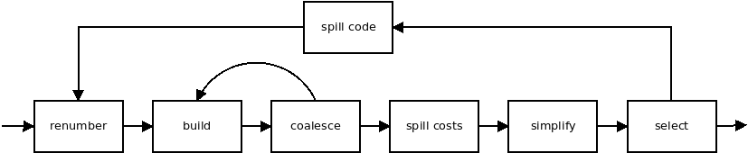
I’ve ignored many things here: Coalescing is the process of merging non-interfering, copy related live ranges together. I will talk later about renumbering.
Live Range Splitting
In the ticket linked above, AndreasK has observed, that live ranges are spilled, even though they may be fit into liveness holes and a coloring could be found, by splitting the LR. What does this mean? Let’s look at the following pseudo-code:
x <- 1 # def x
y <- 1 # def y
loop {
    y <- y + 1  # use y
}

loop {
    # use x
}
Imagine for a moment this code makes sense (or would you rather stare at real assembly?).
If we had only two registers and our heuristic decides to spill either x or y, we’d have an additional load and a store in each loop.
At this point you may say “hold up, there are no loops in Haskell”, or “Why not put the load before the loop and the store after it?”.
Since we’re working on machine instructions at this stage in the compiler, loops do exist - in the form of jumps between blocks.
Choosing which LRs to spill and spill code placement are subjects in their own right. Let’s just say that this example is simplified
and that -fregs-graph places the spill code right around the instructions, later cleaning up unnecessary ones.
I jumped on this and tried to implement Passive Live Range Splitting, by Cooper and Simpson. This algorithm is supposed to figure out, that we can split x like this:
x <- 1 # def x
y <- 1 # def y
STORE x
loop {
    y <- y + 1  # use y
}

LOAD x

loop {
    # use x
}
The paper looked simple and like a great solution, so I went ahead with it.
Jumping the Gun
I wasn’t familiar with the code base (or the algorithm) and did some learning by doing. I’ll give you the quick run down of my revelation:
In my description of live ranges, I made it sound like we are assigning registers to live ranges. That isn’t quite correct. There is no explicit modelling of live ranges (“webs”) in GHC (and probably in most compilers?). We are operating on vregs and those are mapped to physical registers.
Remember that “renumbering” step in the diagram earlier? This is actually about live range discovery.
This whole coloring process is repeated. Like I noted before, spilling technically creates tiny live ranges
and -fregs-graph renames them on-the-fly.
To split live ranges, inserting stores and loads is not enough, you have to rename (“renumber”) the vregs in the instructions,
to reflect the new live ranges!
But -fregs-graph doesn’t have a renumbering phase.
While analyzing this simple reproducing example program, it dawned on me.
I saw something similar to this in assembly:
{
  def x
  use x
  def x
  use x
}
...
{
  def x
  use x
}
There were no branches with different definitions of x. In fact, x was redefined in the same basic block, redefined and used in a later block. Those are disjoint live ranges, but by having the same vreg name, they are constrained to be assigned to the same physical register! We don’t need live range splitting, we need live range discovery!4 I falsely assumed that vreg = live range.5
Things going Sideways
I briefly and desperately tried to create some makeshift renumbering for my split LRs, but it was no use. Figuring out where the new live ranges are and how to name them is hard, even though you technically only have to look “before” your inserted store and “after” the inserted load. But in the presence of control flow (branches and loops), it’s not that simple:
def x
STORE x
if (..) {
  use y
} else {
  LOAD x'
}
use x
Which x should we use after the branches join? This code is wrong and we either need to place a LOAD x' into the if-block,
or possibly a copy x' -> x in the else branch.
To do that, I’d need to build a reaching definition analysis anyway and then some.
Discovering Live Ranges
So I decided to address the problem at hand by implementing a “renumbering” phase.
The “classic” way of doing this, is by performing data-flow analysis to build explicit def-use chains. Basically, we want to find all vreg definitions, create a list for each of them and add all the positions in the program where this definition was used. The data-flow analysis to get the reaching definitions is generally performed by a fixed-point algorithm. Straight line code is simple, but for loops, you have to iterate until your data-flow facts no longer change (i.e., the fixed-point is reached). This due to the fact, that information from the loop body can flow back to the loop head.
Once you have your def-use chains, i.e., n lists for each LR, you’ll want to perform pairwise intersection tests for all lists (with the same vreg). There are probably ways to optimize this, but this takes a lot of time and space!
In fact, it seems like this is not the way to do it anymore. E.g., looking at “Engineering a Compiler”, after giving an overview of the problem it says:
Conversion of the code into ssa form simplifies the construction of live ranges; thus, we will assume that the allocator operates on ssa form.
Even Briggs in 1994 wrote, that their compiler uses SSA instead of the “classical” way that Chaitin used.
SSA - What & Why
What is SSA and how does it help us? An intermediate representation is in Single Static Assignment form, if it conforms to a simple property:
Each name is only defined once, respectively, each definition introduces a new name
This has many nice implications, simplifies data-flow analysis and even enables new optimizations6.
Any use of an SSA-variable x is dominated by its definition, i.e., any path from the start of
the control flow graph of the program to the use has to go execute that definition - and there is only one definition.
Def-use chains are no longer necessary, each definition has to come from a straight line of predecessors, be within the same basic block, or defined by a φ-function at the beginning of a block or come from
What is a φ-function (or φ-node, “phi-function”)?
Let’s say we have a variable x that is redefined several times.
Each time, we update an index to create a new name, i.e., x0, x1, …
What if you have two different definitions of x reaching your basic block?
Which name do you have to choose?
This is where φ-functions come into play. Think of them as magically “selecting”
the right name, depending on where the control flow came from and defining a new name for
the selected value: x2 = φ(x0, x1)
Semantically, these are considered to be executed as parallel copies, all at once,
at the beginning of the block, before the first instruction.
Here some code, which is not in SSA-form:
x := 0
if (...) {
    x := x + 1
} else {
    x := x + 2
}
y := x
…and transformed:
x_0 := 0
if (...) {
    x_1 := x_0 + 1
} else {
    x_2 := x_0 + 2
}
x_3 = φ(x_1, x_2)
y := x_3
SSA Destruction and Live Range Discovery
Naturally, we can’t leave the code like this. CPU’s simply don’t have a φ instruction, we need to get rid of them.
The process of transforming a program in SSA-form out-of-SSA (thus resolving all φ-functions) is sometimes called SSA Destruction. There is quite a bit of literature on this and it gets complicated if you want fast and correct SSA destruction.
But for our case, things are simpler. For now, all we want is to rename our live ranges, so that each vreg represents a single, disjoint live range. Sreedhar et al.7 noted the distinction between Conventional SSA (CSSA) and Transformed SSA (TSSA). A program is in CSSA right after SSA transformation (or after repair) and in TSSA once any program transformations have moved, removed or added code. The difference is, that the φ arguments in CSSA do not interfere - whereas in TSSA they might. Resolving φ-functions with interfering arguments requires the insertion of copies and to keep your program fast, you will want to figure out which ones you need and which ones you can get rid of. For CSSA, you simply gather all names connected by φ-functions, using a union-find (disjoint-set union), then assigning one name to each disjoint set. Voilà, you’re done!
Further Reading
Cooper & Torczon’s “Engineering a Compiler” is one of my favorite textbooks on compilers and contains lots of information on register allocation and SSA.
The (unfortunately unpublished) “SSA Book”, by France’s INRIA, is a real treasure trove and shouldn’t be missed.
For a more exhaustive bibliography, check out Jeremy Singer’s SSA Bibliography.
Conclusion
To summarize, in order to improve GHC’s graph coloring register allocator, I wanted to implement passive live range splitting, but discovered that several disjoint live ranges may bear the same vreg name. I’ve described what SSA is and how it may solve the problem.
In the next part, I’ll describe how I implemented SSA-transformation in GHC and what the results were.
If you spot any mistakes, omissions or want to provide feedback, comments, questions - you can reach me on Twitter, or via mail with my username at gmail.
-
Poletto99. Note that this algorithm is generally extended in such a way, that it isn’t really linear. ↩
-
Technically, this breaks the LR up into many tiny LRs, which still can cause interferences. ↩
-
Confusingly, the literature seems to use live range splitting for both things, I prefer live range discovery to simply rename disjoint live ranges. ↩
-
What do we learn? Always test your assumptions, i.e., check yourself before you wreck yourself! ↩
-
E.g., Sparse Conditional Constant Propagation ↩
-
SreedharJGS99 - “Translating out of static single assignment form.” ↩